Dear Esteemed Reader,
I’ve had the privilege to observe different methods in microtonal, tuning and sound synthesis discourse this past month. Much of it has been in regards to the Plomp-Levelt dissonance curve and its implications about how we perceive harmony.

This plot represents the amount of dissonance between two frequencies. The first being the frequency/note, or “C” at the origin, and the second being variable across the whole graph. The value range from 1 to 2 on the x-axis represents the ratio between that first note and the second variable frequency. What’s important to note is where the local minima, or dips appear. These dips correlate exactly with the intervals mentioned two blog posts ago:

This curve originated from subjective data, asking participants to rate dissonance between intervals they heard; this experiment originated with Hermann von Hemholz’s On the Sensations of Tone as a Physiological Basis for the Theory of Music (1863) and has been replicated. A significant criticism for earlier experiments is lack of cultural diversity among participants giving results that reflect just intonated western music. Although this is thoroughly addressed in Plomp and Levelt’s Tonal Consonance and Critical Bandwidth (1965), their results still reflect the western major scale. There has been recent work in modeling this curve and I’ve been using William Sethares’ 2nd order ODE based model to yield more of the intervals listed above, common in Indian classical music, and Maqam theory.
The value of dissonance curves is that it gives intervals a value for how harmonious they are, aiding my Xenharmonic MIDI tuner for narrowing down tuning options. This model takes the timbre of a sound into account so the dissonance between its overtones can be considered as well, yielding complex scales and relationships. Currently, I’m expanding on the model to handle polyphonic harmony rather than just two notes for the Xenharmonic MIDI tuner. In the future, I will review different dissonance curve equations and perform a meta analysis comparing their contours to other studies of dissonance, ranging from neural noise reactions (https://journals.aps.org/prl/abstract/10.1103/PhysRevLett.107.108103) to suggested formulas from the renaissance (https://en.xen.wiki/w/Benedetti_height) to current day (https://en.xen.wiki/w/Chord_complexity#Generalized_Tenney_and_Weil_Heights:_Span-Corrected_Dirichlet_Complexity ) and update the Xenharmonic MIDI tuner if need be, noting relations to the tonal mappings mentioned in an earlier blog post.

I’m considering a DIS (Research Directed Individual Study) as a means to continue studying and composing xenharmonic music. Here is a polished sample of what I’ve written: https://musescore.com/user/57762682/scores/26949583?share=copy_link. I’ve been recruited to collaborate and compose with iGEM for a global competition in October and my Lumatone has arrived just in time for returning back to FSU. I intend to present it and my compositions during a time slot at the presidential showcase in October. Xenharmonically composing this summer has pushed my ear and creativity further away from a purely 12 tone framework preparing me to jump into 24, 31, and 53 toned systems and not rely on the quazi-12 tone nature within them, nor have my attempts to break out be blind and arbitrary. Funnily, I anticipated the inverse if not for mailing holdups.
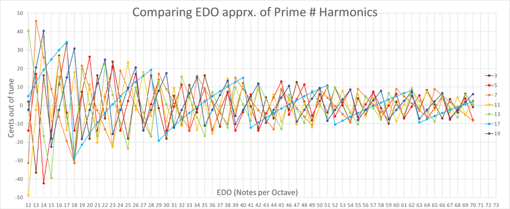
This graph highlights why some # of note systems would be prioritized over others. As the amount of notes increases, the error of approximation approaches zero, however may become unwieldy to play. For my purposes, the lower prime harmonics are prioritized over the higher numbered ones, predominantly 3, 5, and 7. I’m excited to hear and feel these differences for myself.
